Rendering the connectome in 3-D

connkg quilt and connkg viz3d draw a connectome where it is: every neuron at its real position in the brain. Other 3-D views in the KGRAG fleet grow an invented tree layout. A connectome does not need one, because the microscope already put every neuron somewhere.

Two views are available:

• Circuit (--view circuit, the default) draws the traced skeletons of the neurons that one or more SPECs resolve to.
• Flow (--view flow) draws neuropils as spheres, linked by tubes weighted by how much signal the brain's neurons carry between them.

Both views draw the whole brain as a context cloud behind the subject, and, once fetched with connkg meshes, the brain's neuropils as faint surfaces. Both render either as a Looking Glass quilt or in an interactive viewer.

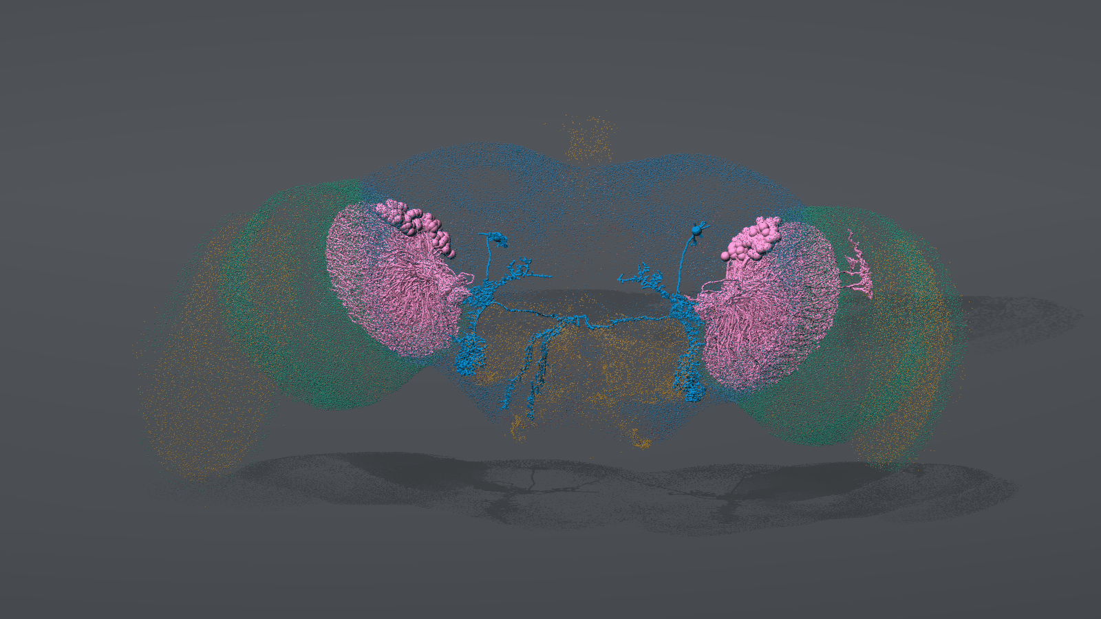
The escape circuit in its anatomy. Pink is LPLC2, the looming detectors, whose dendrites fill the lobula of each optic lobe; blue is DNp01, the giant fiber, which collects from them in the central brain and sends the two axons leaving the bottom of the frame down to the nerve cord. Behind them the 78 neuropil surfaces, and one dot for each of the 139,255 neurons, placed at its cell body. Both populations come from a spec the query layer understands: connkg quilt LPLC2 DNp01 --tubes --cloud. See Reading the images.

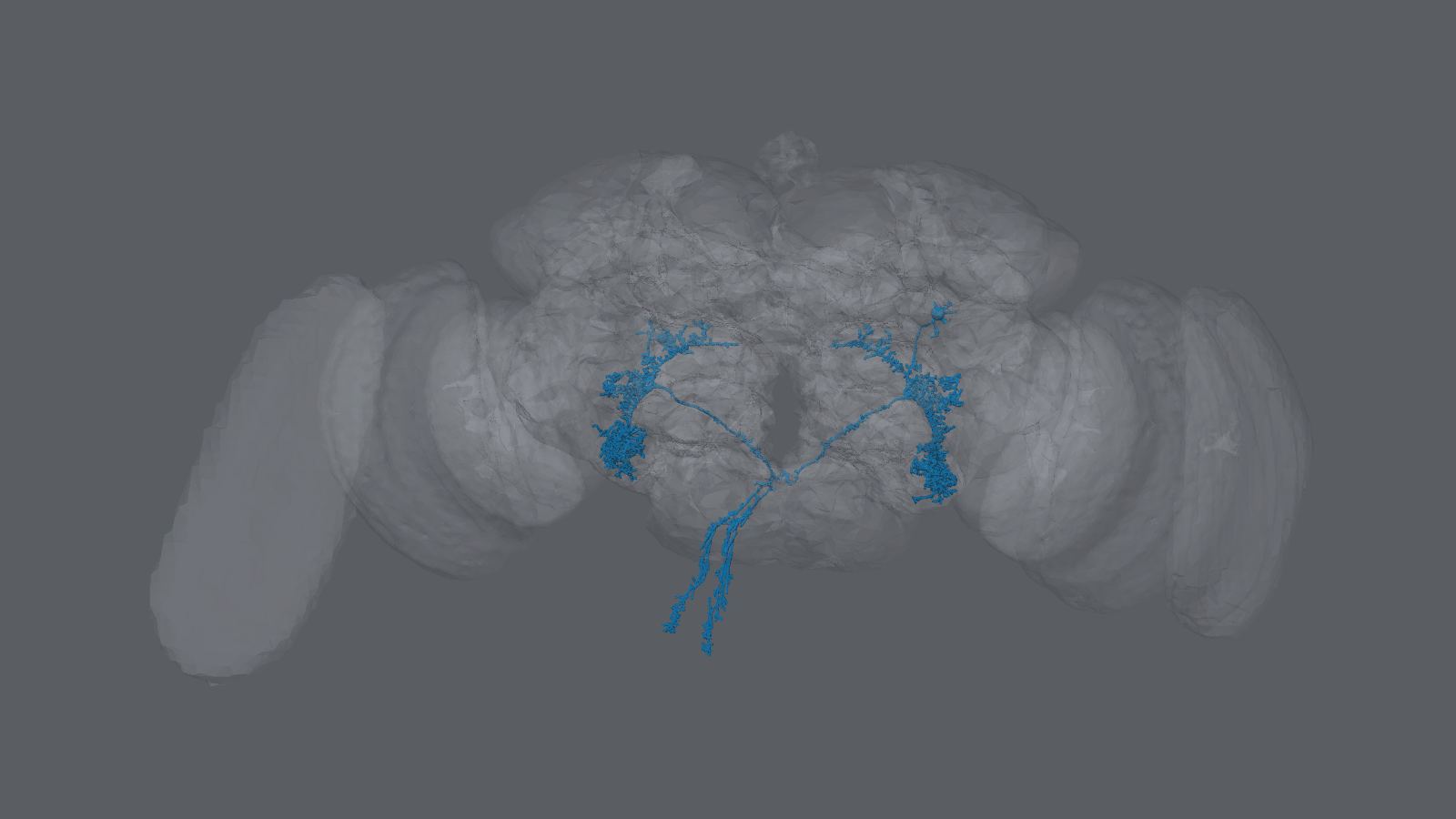
Circuit view: the two DNp01 giant fiber neurons, drawn from their traced skeletons, inside the FAFB v783 neuropil surfaces. Drawing the surfaces turns the whole-brain cloud off, which is why there are no dots here and the optic lobes read as layered shells. See Reading the images.

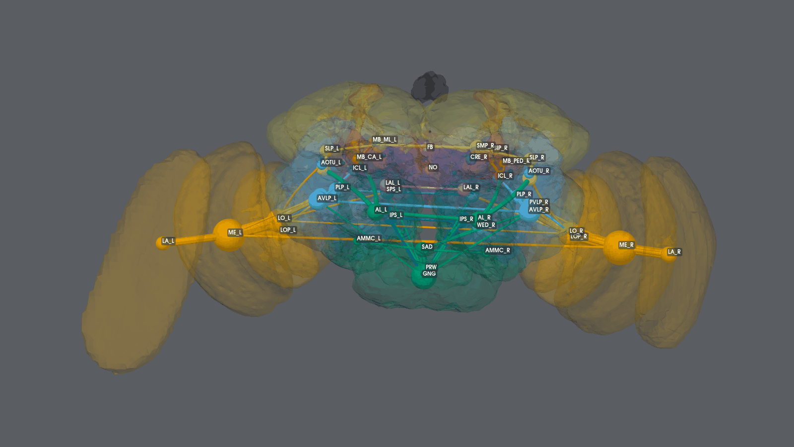
Flow view: the strongest 100 of 5,786 directed neuropil pairs, with each neuropil labeled. See Reading the images.

Data credit and license

The images on this page are renders of the FlyWire FAFB v783 connectome: Dorkenwald, S. et al. (2024), Nature 634, 124-138, and Schlegel, P. et al. (2024), Nature 634, 139-152. The data is licensed under CC BY-NC-SA 4.0. The renders are adaptations of it, shared under the same license, not under the software's Elastic License 2.0.

Reading the images

Every image on this page has the same three layers: a gray background, the context cloud, and the subject of the view. The keys below give what each color, shape and size means.

Region and cell-type colors are the saturated Okabe-Ito colors, which stay distinguishable under the common forms of color blindness. The context cloud uses saturated colors too (Okabe-Ito for most super classes, with a wine, indigo and olive for the three smallest), muted part of the way toward the gray background, so the subject of each view stands out from it. No color is a pastel, and shapes and labels back up color wherever the distinction matters.

Background and context cloud

The background is a flat gray, #5A5D62, unless --background or the viewer's Background box says otherwise. It carries no data. The swatches below are for the default gray: the cloud is muted toward whatever background is drawn.

Each small dot is one neuron, at its soma once connkg skeletons has back-filled somas, and at its marked point otherwise.

In the circuit view, all 139,255 neurons are drawn, and a dot's color is the neuron's super class, muted toward the background (the swatches show the colors as drawn):

color	super class	neurons in FAFB v783
#28688E	central	32,381
#28806B	optic	77,873
#578CAC	visual_projection	7,684
#986C87	visual_centrifugal	522
#A7812C	sensory	16,938
#ACA750	sensory_ascending	612
#9D5D2C	ascending	1,750
#733C5A	descending	1,305
#443C76	motor	110
#7C7E48	endocrine	80

The broad regions of the brain follow from these colors. The two large green masses are the optic lobes. The orange arcs outside them are sensory neurons, which are mostly visual: 11,426 of the 16,938 sensory neurons. The blue mass between the optic lobes is the central brain.

With --color-by sign, the dots are colored by transmitter sign instead: #96584D excitatory, #416683 inhibitory, and #7D838A unknown.

In the flow view, every 10th neuron is drawn and every dot is the same gray, #74787E, whatever --color-by says. The cloud there only outlines the brain, so that color in the flow view means one thing: a neuropil's brain region.

Circuit view

what you see	what it means
Branching lines in one color	The traced skeleton of each neuron of one cell type. Every cell type has its own color.
A sphere in the same color, on the skeleton	That neuron's soma (cell body), or the skeleton's root point if the skeleton has no soma.
A larger sphere in the same color, away from any skeleton	A neuron with no skeleton file, drawn at its marked point.
Tubes instead of lines	The same skeletons, drawn with --tubes.
A floor and a shadow under the brain	--floor. The shadow shows depth. It carries no data.

A cell type's color is one of the seven non-black Okabe-Ito colors, fixed by its name, so it is the same in every render. The color identifies the type within one image; it does not encode a category, and it can match a super class color in the cloud. In the images on this page, DNp01 is #0072B2 and LPLC2 is #CC79A7.

Flow view

what you see	what it means
A large sphere with a label	A neuropil, placed at the synapse-weighted center of its neurons. _L and _R mark the left and right hemisphere; a name with no suffix spans the midline.
Sphere color	The neuropil's brain region (table below).
Sphere size	The neuropil's synapse count. Radius grows with the cube root, so a sphere twice as wide holds about eight times the synapses.
A tube between two spheres	Signal flow from one neuropil to the other, carried by neurons that take input in the first and make output in the second. See What flow measures.
Tube thickness	The amount of flow, relative to the strongest drawn tube. Radius grows with the square root, so a tube twice as thick carries about four times the flow.
Tube color	The brain region of the source neuropil: the flow leaves a neuropil of that region.
Which way a tube curves	The direction of flow. Seen from above, every tube bows to the right of its direction of travel. In the front view, a tube running left to right bulges toward you and one running right to left bulges away.
A small, darker sphere with no label	A neuropil with no drawn tube, shown for context.

Neuropils are grouped into brain regions after the systematic nomenclature FlyWire's neuropils follow (Ito et al. 2014). There are 13 regions and 8 colors, so regions that neighbour each other in the brain share a color:

color	regions and their neuropils
#E69F00 orange	optic lobe: LA, ME, AME, LO, LOP
#56B4E9 sky blue	ventrolateral neuropils: AOTU, AVLP, PVLP, PLP, WED
#D55E00 vermillion	mushroom body: MB_CA, MB_PED, MB_VL, MB_ML
#CC79A7 reddish purple	central complex: FB, EB, PB, NO; lateral complex: BU, LAL, GA
#F0E442 yellow	lateral horn: LH; superior neuropils: SLP, SIP, SMP
#0072B2 blue	inferior neuropils: CRE, SCL, ICL, IB, ATL; ventromedial neuropils: VES, EPA, GOR, SPS, IPS
#009E73 bluish green	antennal lobe: AL; periesophageal neuropils: SAD, AMMC, FLA, CAN, PRW; gnathal ganglia: GNG
#000000 black	ocellar ganglion: OCG; unassigned: UNASGD

connkg quilt and the viewer draw the spheres without labels, so use the region colors there. The images on this page add labels, which tell apart neuropils that share a color.

Neuropil abbreviations in the images on this page

label	neuropil	region	color
AL	antennal lobe	antennal lobe	#009E73
AMMC	antennal mechanosensory and motor center	periesophageal neuropils	#009E73
AOTU	anterior optic tubercle	ventrolateral neuropils	#56B4E9
AVLP	anterior ventrolateral protocerebrum	ventrolateral neuropils	#56B4E9
CRE	crepine	inferior neuropils	#0072B2
FB	fan-shaped body	central complex	#CC79A7
GNG	gnathal ganglia (subesophageal zone)	gnathal ganglia	#009E73
ICL	inferior clamp	inferior neuropils	#0072B2
IPS	inferior posterior slope	ventromedial neuropils	#0072B2
LA	lamina	optic lobe	#E69F00
LAL	lateral accessory lobe	lateral complex	#CC79A7
LH	lateral horn	lateral horn	#F0E442
LO	lobula	optic lobe	#E69F00
LOP	lobula plate	optic lobe	#E69F00
MB_CA	mushroom body calyx	mushroom body	#D55E00
MB_ML	mushroom body medial lobe	mushroom body	#D55E00
MB_PED	mushroom body pedunculus	mushroom body	#D55E00
ME	medulla	optic lobe	#E69F00
NO	noduli	central complex	#CC79A7
PLP	posterior lateral protocerebrum	ventrolateral neuropils	#56B4E9
PRW	prow	periesophageal neuropils	#009E73
PVLP	posterior ventrolateral protocerebrum	ventrolateral neuropils	#56B4E9
SAD	saddle	periesophageal neuropils	#009E73
SIP	superior intermediate protocerebrum	superior neuropils	#F0E442
SLP	superior lateral protocerebrum	superior neuropils	#F0E442
SMP	superior medial protocerebrum	superior neuropils	#F0E442
SPS	superior posterior slope	ventromedial neuropils	#0072B2
VES	vest	ventromedial neuropils	#0072B2
WED	wedge	ventrolateral neuropils	#56B4E9

Quilts and Looking Glass displays

A Looking Glass display shows a 3-D scene without glasses. Lenticular optics send a slightly different image toward each viewing angle, so each eye sees the scene from its own position. The display plays a quilt: a single PNG that tiles many renders of the same scene in a grid, one per camera position.

ConnectomeKG does not build quilts itself. It composes a PyVista scene, and quiltwright renders that scene into a quilt, reports its depth budget, and sends it to the display. For each view, quiltwright:

1. Starts from the scene's camera. The camera's focal point becomes the plane of the physical glass. ConnectomeKG places the focal plane inside the brain (see Camera and framing), so nearer structures stand in front of the glass and farther ones sit behind it.
2. Slides the camera sideways across the display's view cone without turning it.
3. Renders with an off-axis (asymmetric-frustum) projection, which keeps the glass plane identical in every view. The display can only fuse views that share that plane. Turning each camera toward the subject ("toe-in") produces ghosting instead of depth.

The default preset, 16-landscape, targets the 16-inch landscape display: 48 views in 8 columns and 6 rows, and a 7680 x 4320 quilt. The display accepts a 50-degree view cone, but connkg quilt sweeps 35 degrees by default (--view-cone), the same cap quiltwright's own CLI applies. View 0, the leftmost camera, is the bottom-left tile. The filename suffix, for example _qs8x6a1.77778, records the columns, rows and aspect ratio, so Looking Glass Bridge configures playback from the name.

A scene that is too deep for the display looks blurred at its front and back. The depth budget is how far in front of and behind the glass plane a scene can extend before that happens. connkg quilt checks it on every run (see World coordinates).

For the full method, the other rendering backends, and Bridge setup, see the quiltwright documentation, in particular the PyVista backend.

Before you begin

You need the following:

• The viz3d extra, which installs PyVista, PyQt5, pyvistaqt and quiltwright:

  pip install -e ".[viz3d]"      # or: poetry install --extras viz3d
  

• A built graph in connectomes/<dataset>/.connectomekg/graph.sqlite. See the README for connkg build and --dataset.

• For the circuit view, skeletons -- from either source, the cache first:

  • The skeleton cache, .connectomekg/skeletons/, written once by connkg skeletons --data-dir fafb_v783 -j 12. It holds every neuron's simplified skeleton in 2.5 GB, so a render needs neither the 31 GB nor an SWC parse. See The skeleton cache.
  • The skeleton download in fafb_v783/sk_lod1_783_healed/, one .swc file per neuron, about 31 GB. Any neuron the cache does not hold is read from here when --data-dir is given.

  With neither, each circuit neuron is drawn as a sphere at its marked point. The flow view does not read skeletons. - For the neuropil surfaces, the mesh cache. Fetch it once with connkg meshes, which downloads the 78 FAFB v783 neuropil meshes from FlyWire's public bucket (no sign-in, about 1 MB) into connectomes/<dataset>/.connectomekg/neuropil_meshes.npz. Without it, both views are drawn without surfaces. See Neuropil meshes.

Render a view

A SPEC is a cell type name (LC4), a root id, a neuron node id, or label:<regex> over community labels. Specs are case-sensitive.

To open a view in the interactive viewer, run connkg viz3d:

connkg --root . viz3d                           # circuit:compass, then explore
connkg --root . viz3d LC4 DNp01                 # circuit: two cell types
connkg --root . viz3d --view flow               # flow: whole brain
connkg --root . viz3d --view flow LC4           # flow carried by LC4 only

Drag to orbit, scroll to zoom, and shift-drag to pan. The viewer also picks neurons, re-resolves specs in place and toggles what is drawn -- see Using the viewer below.

To render a quilt without a window, run connkg quilt:

connkg --root . quilt DNp01 --preview dnp01.png
connkg --root . quilt --view flow --top 60 --floor --cast

To render one flat image instead of a quilt, add --still. The still is the quilt's center view at the preset's aspect, 3840 x 2160 for 16-landscape:

connkg --root . quilt LPLC2 DNp01 --tubes --floor --still

connkg quilt prints what it drew and, for a quilt, a depth report. It then writes files under renders/:

path	contents
renders/stills/	a --still image, and the --preview PNG when the value is a bare filename
renders/quilts/	the quilt, named after the specs (flow_LC4_qs8x6a1.77778.png for a flow)

Quilts are never committed.

Options

option	views	default	effect
--view	both	circuit	circuit or flow
--color-by	both	super_class	context cloud color: super_class or sign
--data-dir	circuit	fafb_v783	skeleton download root
--skeleton-step	circuit	4	keep every Nth skeleton point, 1 to 50
--tubes	circuit	off	draw skeletons as tubes instead of lines
--top	flow	100	strongest neuropil pairs drawn, 1 to 500
--neuropils / --no-neuropils	both	on	draw the neuropil surfaces, when connkg meshes has fetched them
--cloud / --no-cloud	both	on with --floor; else on unless the surfaces are drawn	draw the context cloud
--floor	both	off	stand the scene over a floor lit from above, with shadows
--elevation	both	25 with --floor, else 0	degrees to tilt the camera up so it looks down, -80 to 80
--background	both	gray	gray, charcoal, black, navy, light, or #RRGGBB; the cloud mutes toward it and the floor shades from it
--preset	both	16-landscape	quiltwright quilt preset (8 x 6 views)
--view-cone	quilt	35	degrees the quilt cameras sweep
--fov, --zoom	quilt	14.0, 1.0	per-view field of view in degrees, and camera dolly
--still	quilt	off	render one flat center view instead of a quilt
--cast	quilt	off	send the finished quilt to Looking Glass Bridge; not with --still
--width, --height	viewer	1400, 900	window size in pixels

The circuit view needs at least one SPEC. In the flow view, SPECs are optional.

Using the viewer

connkg viz3d opens a workspace: a control rail down the left side, and the scene beside it with a neuron inspector below. Everything here is per-session -- the viewer never writes to the graph.

Given no SPEC it opens on circuit:compass, so there is a circuit to orbit and pick at from the start; any SPEC replaces it. On a connectome whose cell types that circuit does not name, it opens on the brain alone.

The control rail

The rail holds everything that changes what is drawn, top to bottom: the Dataset and View boxes, the Show box and its Show scene button, an Explore and a Display tab, and Cast to Looking Glass pinned at the bottom where a long tab never pushes it off-screen.

Dataset lists every dataset built under --root, and is hidden when there is only one. Switching opens that graph and closes the old one. The Show box's specs are kept where they resolve in the new graph. Cell type names differ between connectomes, so where they do not, the viewer falls back to what it opens on. View switches between the circuit and flow views, keeping the specs, and frames the new view afresh.

Explore lists every documented spec, answer and named circuit as a button that fills the Show box and draws it, grouped as Circuits, Specs and Answers. The grammar can be explored without being retyped, and a button takes the same path a typed spec does, refusals included.

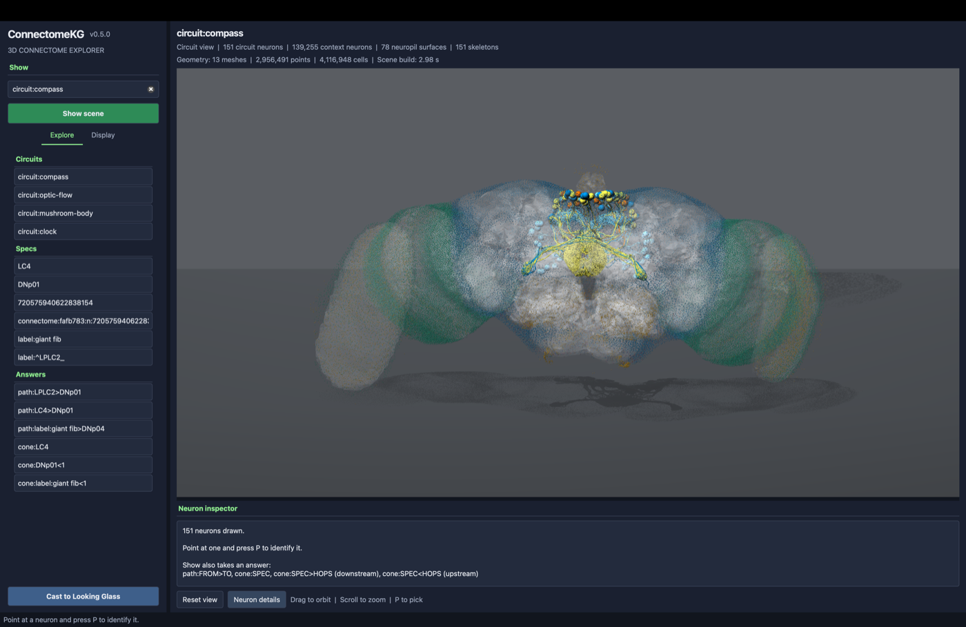
Above: circuit:compass drawn inside the whole brain, the Explore tab listing the circuits, specs and answers, and the inspector reporting what was drawn.

Point at a neuron and press P

Hover the cursor over a drawn neuron and press P. The inspector below the scene names it, gives the description the graph already stores, and lists its strongest partner cell types in each direction. It opens on a pick even if you had collapsed it, and Neuron details collapses it again to give the scene the full height. The flow view draws no neurons, so it hides the inspector entirely.

Picking is bound to a key rather than a left click because a left click is where VTK begins a rotation: picking there would re-answer the question on every orbit.

A pick more than 25 microns from any drawn neuron is reported as a miss rather than as whichever neuron happened to be nearest, so pointing at empty space says so.

Why a click cannot answer this by itself

A whole cell type is drawn as a single actor, so VTK can report which type was hit but never which neuron -- and the neuron is the question. connectomekg.picking carries identity beside the geometry instead: every drawn point paired with the neuron that owns it, resolved by nearest-point lookup. That costs about 12 MB for a 212-neuron scene and 4.4 microseconds a pick, and it is indifferent to --tubes, to the simplification stride, and to whether VTK propagates point data through its filters.

The Show box

The Show box takes the same specs the command does, plus the answer forms from Asking the graph a question, and redraws in place. Press Return or click Show scene. Typing

path:LPLC2>DNp01

replaces the scene with that path, hop-colored. Exploring no longer means restarting, and Cast to Looking Glass follows what is currently shown rather than the specs the window opened with.

Specs are separated by spaces, so a label spec, whose pattern may itself contain spaces, is the one case needing care:

typing	shows
LC4 DNp01	two cell types
label:giant fib	one label pattern -- a leading label: takes the whole box
"label:giant fib" LC4	that pattern and LC4: quote the label to combine it
label:\bgiant\s+fib	backslashes reach the regex unescaped

A spec matching nothing, an unclosed quote, or a spec over the scene cap is refused with the reason, and the scene is left as it was -- including when only one spec of several is bad, since drawing the rest would look like a scene that contained them all. A refusal opens the inspector to explain itself.

What the scene reports

Above the scene sit its title and two summary lines. The first counts what was asked for: the view, the circuit and context neurons, the neuropil surfaces, and the skeletons drawn -- or the flow arcs, in the flow view.

The second counts the geometry that reached the renderer: visible meshes, points and cells, after glyphs and tubes have expanded into real meshes, with a per-group breakdown in its tooltip. Cells are mesh faces, lines, vertices or strips -- not neurons, and not GPU triangles. It is the number to watch when a scene turns sluggish; the tooltip names the usual remedies, which are hiding the cloud or the surfaces, turning tubes off, or raising the stride.

Scene build on that line times the composition on your machine, from the first query to a framed scene. It is a build cost, not a frame rate and not a cast duration.

The Display tab

control	what it does
Whole-brain cloud	one dot per neuron at its cell body; see below
Neuropil surfaces	the 78 meshes connkg meshes fetches
Floor and shadow	stands the scene on a lit floor
Skeletons as tubes	draws skeletons as tubes rather than lines
Skeleton stride	detail, where 0 means choose it from the neuron count
Minimum synapses	drops connections below the threshold
Background	the scene background: Gray, Charcoal, Black, Navy, Light, or Custom for any color

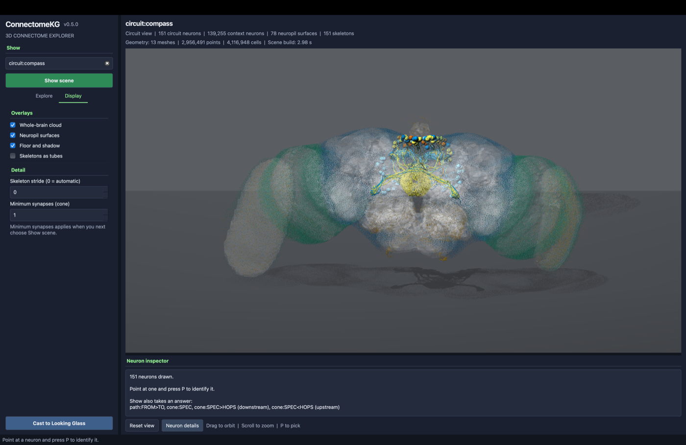
The cloud toggle has three states rather than two. Checked always draws it, unchecked never does, and the third -- partially checked -- is automatic: draw the cloud only when no neuropil surfaces are available, which is what a fresh viewer does when connkg meshes has not been run. Automatic is a state the viewer keeps, so changing some other setting will not quietly decide the question for you.

Background redraws the scene the same way a toggle does, keeping the camera. Saved images, quilts and casts use it too. The default gray suits the region colors. Charcoal and Black show them at their most saturated, but hide the black spheres of nerves and the cervical connective. Navy is a deep blue, #14213D, dark enough that the blue regions still stand off it. Light is for print.

Minimum synapses is what makes a multi-hop cone usable interactively: cone:LC4>2 is 19,866 neurons at the default and 104 at 200. Unlike the toggles it is read when specs are next resolved, so it takes effect on the next Show scene, not the moment it changes -- the rail says so beneath it.

Each toggle redraws rather than hiding an actor, because the overlays are composed: the cloud is one glyph per neuron and the surfaces are 78 merged meshes, so keeping both around to flip visibility costs more than rebuilding without them. A toggle keeps the camera where you put it -- it changes what is drawn, not what is being looked at -- while a new spec or answer re-frames, since the old camera may not contain it.

Reset view, under the scene, frames the current scene again, undoing an orbit or a zoom.

While a scene composes, the rail and the scene are disabled and the cursor turns to a wait cursor. Composing runs on the GUI thread and pumps the event loop to stay responsive, which also delivers clicks; disabling the controls is what stops a second composition from starting on top of the first.

Saving the scene

Save scene..., above the cast button, writes what you are looking at without a Looking Glass in the loop. Image renders one 4K still, framed and lit the way connkg quilt --still renders, floor and shadows included; Quilt writes the quilt that Cast would send, at the --preset the viewer opened with. Both re-compose the scene off-screen from the current specs, display settings and camera, so the file matches the viewport rather than being a screen grab of it.

The dialog opens in renders/stills/ or renders/quilts/ with the scene's name filled in. The name you choose is the stem: quiltwright appends the spec suffix that Looking Glass readers and the render scripts rely on, so saving compass.png as an image writes compass_qs1x1a1.77778.png, and as a quilt compass_qs8x6a1.77778.png. The path actually written is shown in the status bar. A web-page export is not offered: the scene's point cloud alone is hundreds of megabytes once serialized into a page.

Casting to a Looking Glass

Click Cast to Looking Glass to send the current camera view as a quilt. Looking Glass Bridge must be running; see Set up Bridge and the display.

How a scene is built

Every render path calls one function, connectomekg.scene.build_brain_scene. It composes the scene into a PyVista plotter that the caller supplies. connkg quilt passes an off-screen plotter, the viewer passes its Qt widget, and Cast to Looking Glass rebuilds the scene in a fresh off-screen plotter. All three therefore draw the same thing.

The function works in five steps:

1. Set the background to a muted gray (scene.BACKGROUND, #5A5D62).
2. Compute the world frame from the neuron positions.
3. Draw the neuropil meshes, when cached and neuropils=True.
4. Draw the context cloud, unless meshes were drawn (cloud=None, the default) or cloud=False.
5. Draw the circuit or the flow.

The module is split so most of it runs without PyVista. world_frame, context_points, circuit_neurons, neuropil_flow and flow_arc are NumPy and SQL only. The tests exercise them without the viz3d extra.

Data each view reads

data	source	read by
neuron positions	soma_x, soma_y, soma_z in each neuron node's metadata where connkg skeletons back-filled one, else x, y, z -- the Codex marked point on FAFB, the soma on BANC and MCNS -- in nm	world frame, context cloud, flow centroids
super class and sign	neuron node metadata	context cloud color
skeletons	.connectomekg/skeletons/ (written by connkg skeletons), then fafb_v783/sk_lod1_783_healed/<root_id>.swc for whatever it does not hold	circuit
per-neuron neuropil synapse counts	IN_NEUROPIL edge evidence, {"pre": n, "post": m}	flow
neuropil synapse totals	neuropil node metadata, n_synapses	flow sphere size
neuropil surfaces	.connectomekg/neuropil_meshes.npz, written by connkg meshes	both

World coordinates

FAFB coordinates are image coordinates in nanometres: x runs across the brain, y increases ventrally, and z runs through the section stack. The 3-D stack expects +z up.

build_brain_scene centers the scene on the median neuron position and scales it to 1 world unit per 100,000 nm. It maps each point as follows:

world = ((x - cx) / S,  (z - cz) / S,  -(y - cy) / S)       S = 100,000 nm

Negating y puts dorsal up. At this scale the brain is about 8 x 4 x 3 world units, which fits inside the depth budget of a Looking Glass quilt.

Marker sizes are in world units too, set on FAFB v783, so another dataset needs them scaled. world_frame measures the dataset's framed extent: the larger of its neurons' 1st-99th percentile width divided by 16:9 and their height, which is what the camera fits to a landscape frame. It divides that by FAFB's 410,000 nm, clamped to 1-4, and neuropil spheres, flow tubes and soma spheres are multiplied by the result (WorldFrame.marker_scale). The context cloud keeps FAFB's size, because scaled-up dots speckle the spheres inside them.

Camera and framing

connectomekg.scene.aim_camera sets the camera in three steps:

1. kg_utils.viz3d.frame_tree points the camera along world +y, so you see the brain from the front with dorsal up.
2. With a non-zero --elevation, the camera tilts up by that many degrees and looks down on the brain.
3. quiltwright.frame_and_focus fits the scene tightly at that final direction and puts the focal plane at the harmonic mean of the scene's near and far depths. A tilted view framed by reset_camera() instead leaves the brain small in frame.

frame_and_focus fits to the window's shape, so connkg quilt sizes its window to the aspect quiltwright captures each view at (16:9 for 16-landscape), not to the quilt tile (4:3). After framing, the camera is fixed: the depth report and the render both take fov=None, so neither re-frames it.

For a quilt, connkg quilt prints quiltwright.depth_report for that camera and --zoom. The report lists how many pixels the nearest and farthest geometry shift between neighbouring views. Around 4 to 5 px is the practical ceiling, and rows above 5.5 px are flagged as soft. The flow view with a floor comes to about 3.4 px at --zoom 1.0 and about 3.7 px at --zoom 1.1. Above about 1.15 the camera crops the optic lobes, because the brain already spans the width of the frame.

The context cloud

The context cloud draws each neuron as a small sphere. The cloud shows the outline of the brain: optic lobes, central brain and the gaps between regions.

Each sphere sits at the neuron's soma where the graph has one -- soma_x/soma_y/soma_z, written by connkg skeletons -- and at its marked point otherwise. A graph without the back-fill draws the marked-point cloud it always did. The scene's title says which: somas=N once any of the dots is a real cell body, context=N while none is.

Three choices keep it visible without covering the subject:

• Spheres sized in world units, not pixels. A 2-pixel point disappears in a Retina window and in a quilt tile. A world-sized sphere scales with the camera like the rest of the scene. Each sphere is a low-poly glyph (6 x 4 facets), so the full 139,255-neuron cloud is about 3.3 million triangles and composes in under a second.
• Muted, opaque colors. Each dot's color from connectomekg.colors is blended 45% toward the gray background (_CONTEXT_MUTE). The hue stays, but the skeletons and neuropils drawn at full saturation stand out, even where a cell type shares a hue with the dots around it. The blend goes toward the background, not toward white, because lightened colors turn pastel and color-blind readers cannot tell pastels apart. The dots are opaque, because alpha blending ghosts between views in a light-field render.
• Thinner and gray in the flow view. The flow view draws every 10th neuron, with larger spheres (radius 0.014 world units, against 0.005 in the circuit view), all in one neutral gray. At full density, the cloud hides the neuropil spheres inside it, and super-class colors would compete with the region colors.

Background and context cloud lists every color.

A marked point is not a cell body: FlyWire's anchor can sit tens of microns from the soma, so a cloud drawn from marked points shows where neurons are rather than where their cell bodies are. connkg skeletons is what replaces them -- see The skeleton cache.

Neuropil meshes

The neuropil meshes are the surfaces of the volumes FlyWire used to assign each v783 synapse to a neuropil: the JFRC2 template neuropils (Ito et al. 2014) mapped into FlyWire space. So a mesh encloses the synapses that the graph's IN_NEUROPIL edges count for that neuropil. FlyWire publishes them as Neuroglancer precomputed meshes at gs://flywire_neuropil_meshes/neuropils/neuropil_mesh_v141_v6. That source numbers the meshes 0 to 77 and does not name them.

connectomekg.neuropil_meshes.FAFB_783_MESH_NAMES names them. It was built by matching every v6 mesh, vertex set for vertex set, against the named copy fafbseg packages from the same source: all 78 match exactly, to 78 distinct names. The one v783 neuropil without a mesh is UNASGD, the synapses no volume claimed. fafbseg's volume_name_dict.json looks like the answer but is not: it numbers the synapse-assignment volume, and matches none of these meshes.

The views draw the meshes like this:

• Circuit view: pale neutral shells, #C8CCD2 at 10% opacity, so the circuit's cell-type colors stay the only color in the scene.
• Flow view: each surface tinted with its brain region's color at 15% opacity, the color its sphere already carries, so the spheres and tubes read as sitting inside their neuropils.

Meshes of one color are merged into one actor (neuropils in the circuit view, neuropils:<color> in the flow view), so the 78 surfaces cost a handful of draw calls. Depth peeling is on so translucent surfaces composite in the right order. On FAFB v783 a 48-view quilt of LPLC2 and DNp01 with meshes renders in about 5 seconds.

The surfaces are the one translucent layer in the scene. Everything else is opaque, because alpha blending can ghost between views in a light-field render. The shells render correctly in every quilt tile, but have not been judged on a Looking Glass display yet. If they ghost, --no-neuropils turns them off.

With the meshes drawn, the context cloud is redundant: the surfaces show the brain's outline more plainly than 139,255 dots. So drawing the surfaces turns the cloud off, leaving the subject inside the anatomy. Pass --cloud for both at once, which is worth it when the dots' own coloring is the point (--color-by sign, say). Without a mesh cache, nothing changes: the cloud draws as it always did.

The skeleton cache

The Codex skeleton download is 31 GB of SWC text, one file per neuron. Two things in it are worth keeping and the rest is not, so connkg skeletons reads every file once and writes both:

connkg --root . --dataset fafb783 skeletons --data-dir fafb_v783 -j 12

-j is the number of worker processes and defaults to 1, which uses one core of however many the machine has. Pass your core count.

• .connectomekg/skeletons/, every neuron's skeleton simplified at --step (4 by default, the circuit view's own default). 2.5 GB on FAFB v783, written as one part-NNNN.parquet shard per worker and read back as one table. The circuit view reads it in place of the download.
• A soma in every neuron node, as soma_x, soma_y, soma_z and has_soma. The context cloud draws somas from then on, and so does any query over the graph. This half writes to graph.sqlite; --no-somas leaves the graph untouched.

Parsing SWC is pure Python and holds the GIL, so the pass pegs one core and leaves the rest idle. -j splits it across processes, each reading a contiguous range of root ids into its own shard. Measured on FAFB v783, 139,255 neurons and 31 GB, on an 18-core laptop (6 performance, 12 efficiency):

workers	wall time	skeletons/s
1	19m 30s	119
12	2m 39s	881

7.4x, and the two caches are identical -- same 212,351,918 points, same 134,675 somas, and the same SHA-256 over a sampled 199 neurons' coordinates, parents and labels. Shards hold disjoint root-id ranges, so a filtered read still skips the ones that cannot match.

It is a one-time maintainer job either way: nothing else in the module needs the download afterwards. Run it again to refresh either product, or after a rebuild. A larger --step trades detail for size.

Every pass writes reports/skeletons_<timestamp>.md, the same per-run provenance record connkg build writes: versions and git commit, options, host, what was read, what was written, timings and peak memory. A failed or interrupted pass writes one too, marked FAILED, and removes its own partial cache. Because the soma back-fill changes an already-built graph, take a fresh connkg snapshot save afterwards -- one taken before the pass measures a graph with no soma_* keys in it.

What the cache holds is not the whole skeleton. It carries no radii, which the renderer does not use, and its only SWC label is the soma's -- branch points and tips are recomputed from the parent links, which is where the renderer took them from in the first place. What it does carry round-trips exactly: a cached skeleton drawn whole is the same geometry as the downloaded one drawn at the cache's stride, to float32 (under 0.03 nm, against a 4 nm imaging voxel). Every measurement above is FAFB v783: 104 LC4 neurons render from the cache in 1.0 s against 1.7 s from the download, with the same 379,096 points. Sharding costs nothing to read -- 252 ms to pull those 104 skeletons out of twelve shards, against 265 ms out of one file of the same size -- because their disjoint root-id ranges let Parquet skip whole shards, and what is left is read in parallel.

Both caches beside the graph -- this one and neuropil_meshes.npz -- are derived data, gitignored, and safe to delete. So is synapse_graph.npz, which connkg path and connkg cone write the first time they load the brain's 3.7 M synapse edges, turning an 8-second load into under one.

The circuit view

The circuit view draws the neurons that the SPECs resolve to, at full brightness:

1. Resolve. Each SPEC goes through ConnectomeKG.neurons_of, and the results are merged without duplicates. A scene holds at most MAX_SCENE_NEURONS (500) neurons. Above that, the render stops with an error that names the count, because a silently sampled circuit looks complete when it is not. Narrow the spec instead.
2. Load skeletons. The cache is read first, and --data-dir covers whatever it does not hold: connectomekg.skeletons.read_swc parses those neurons' SWC files. Both sources are in the graph's own nanometre frame, so skeletons and the cloud line up without a transform.
3. Simplify. --skeleton-step N keeps every Nth point along each unbranched run. Roots, the soma, and every branch point and tip are always kept, so the branching shape stays intact at any step. Branch points and tips come from the parent links, not from the SWC labels, which real skeletons do not apply consistently. A cached skeleton is already simplified at the cache's own stride, so the requested stride is divided by it rather than applied again, and a request below it draws the cache as it stands.
4. Draw. All the neurons of one cell type share a single line mesh (skeleton:<type>), so a 100-neuron type costs one draw call. A sphere marks each soma (soma:<type>).

The mesh holds polylines, not one line per traced edge: connectomekg.skeletons.polylines walks the parent links and returns each unbranched run between one branch point (or root) and the next branch point (or tip). Both carry the same edges, but --tubes extrudes a line mesh, and extruding disconnected edges gives one short cylinder per edge meeting its neighbours at an angle with nothing joining them -- a heap of faceted stubs rather than a neuron. Tubing a run instead gives one continuous surface with mitred joins, and costs less: a run's interior points are shared rather than repeated once per edge. On circuit:compass that is 2.8 M cells against 3.4 M for the per-edge form, while doubling the tube's sides from 6 to 12.

A tube's radius is the traced radius at each point, clamped between the width every skeleton used to be drawn at and the width of the sphere that marks a soma. The floor is there because FAFB's median traced radius is 222 nm, a thread at whole-brain framing: the old constant was doing visibility work, so keeping it as a floor means nothing draws thinner than it did and only thicker structures widen from it. The ceiling is there because the giant fiber, the thickest axon in the brain, otherwise tapers to 13 times the floor and 2.6 times the soma sphere -- a neurite drawn fatter than its own cell body, which reads as a blob rather than an axon. Clipping costs 0.6% of DNp01's points and nothing on a scene like circuit:compass, whose widest point is already under 3.4x the floor. A cache written before the radius column existed (format 1) reads back zeros and draws at the constant width, so a rebuild is what turns the taper on.

Each cell type's color comes from the seven non-black Okabe-Ito colors, indexed by seed_from_key(type name). The same type has the same color in every render and every session. The color identifies the type; it does not encode a category.

Two fallbacks keep a neuron visible when data is missing, and the command output counts both:

• Missing skeletons: a neuron with no SWC file is drawn as a larger sphere at its marked point (fallback:<type>). The larger size marks it as a stand-in, not a measured soma.
• Soma fallbacks: in 3.3% of FAFB v783 skeletons (4,580 of 139,255) no row is labeled soma, so the soma sphere sits at the skeleton's root point instead.

The flow view

The flow view shows how signal moves between brain regions, summed over neurons.

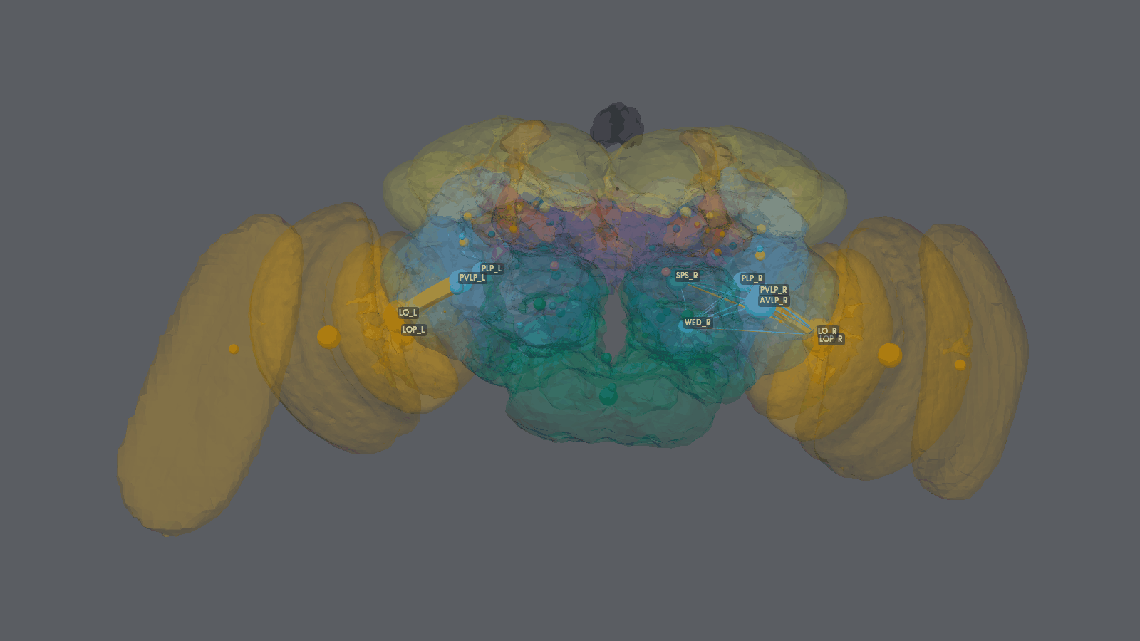
Flow carried by LC4 only. About 90% of it runs from the lobula (LO) to the posterior ventrolateral protocerebrum (PVLP) on each side. See Reading the images.

What flow measures

Each synapse lies in one neuropil. The neuropil breakdown on a synapse edge records where two neurons meet, not how signal moves from one region to another. Signal crosses from neuropil A to neuropil B inside a single neuron that takes input in A and makes output in B.

For each neuron n, the IN_NEUROPIL edges give post_n(A), the input synapses n receives in A, and pre_n(B), the output synapses n makes in B. The flow from A to B is:

F(A -> B) = sum over neurons n of   pre_n(B) * post_n(A) / post_n(total)      A != B

In words, each neuron's output synapses in B are split across neuropils in proportion to where that neuron takes its input, and the result is summed over all neurons. The unit is output synapses.

For example, suppose a neuron takes 30 input synapses in A and 10 in B, and makes 20 output synapses in B and 40 in C. Three quarters of its input is in A and one quarter is in B, so it contributes:

pair	contribution
A -> B	20 x 0.75 = 15
A -> C	40 x 0.75 = 30
B -> C	40 x 0.25 = 10

Flow within one neuropil (A -> A) is left out. A neuron with no input synapses contributes nothing, because its output cannot be attributed to a source.

Keep three limits in mind when you read a flow picture:

• Flow counts synapses, not activity. A strong tube means many synapses sit on that route, not that the route is active.
• Transmitter sign is ignored. Excitatory and inhibitory synapses add together.
• The split assumes that a neuron's output draws evenly on all of its input. That approximation fits a compact neuron better than a neuron with separate input and output compartments.

What is drawn

• Neuropil spheres sit at the synapse-weighted centroid of the marked points of every neuron in that neuropil. The centroids always use every neuron, even when SPECs restrict the flow, so a neuropil sits in the same place in every flow render. A sphere's radius scales with the cube root of the neuropil's synapse count, up to 0.22 world units. A centroid is a position, not the neuropil's shape: the Codex download has no neuropil meshes.
• Color is the neuropil's brain region, from connectomekg.neuropils.NEUROPIL_REGION and connectomekg.colors.REGION_COLOR, so LO_L, LO_R and ME_L are all optic-lobe orange. Spheres and tubes are lit more evenly than the rest of the scene (_FLOW_AMBIENT), because shading darkens a color toward its neighbours: a shaded yellow reads as orange. The images in these docs add neuropil labels; connkg quilt and the viewer do not draw labels.
• Tubes follow the --top strongest pairs. A tube's radius scales with the square root of its flow relative to the strongest drawn pair, and its color is the source neuropil's color.
• Direction shows in the curve. Each tube bows to one side of the line between its endpoints, along the cross product of that line and world up, so A -> B and B -> A curve to opposite sides instead of overlapping.
• Idle neuropils, those with no drawn tube, are drawn at half size and darker.
• Scale follows the dataset. The sizes above were set on FAFB v783. A dataset that fills more of the frame has its spheres and tubes scaled up by the ratio, so they are the same size on screen: 2.32x on BANC v888, whose brain and nerve cord stand 2.3 times as tall as FAFB's brain, and 1.12x on MCNS v1.0. See World coordinates.

Restrict flow to a population

When you pass SPECs with --view flow, only those neurons count toward the flow. For example, connkg viz3d --view flow LC4 shows where the 104 LC4 neurons carry signal. The flow view has no neuron limit, because it draws only neuropils and tubes, never individual neurons.

Scale and cost on FAFB v783

neuropil_flow reads 421,132 IN_NEUROPIL edges and 139,255 neuron positions. It aggregates 138,584 neurons into 5,786 directed pairs across 79 neuropils in about 1.5 seconds, so the flow is computed at render time and nothing extra is stored in the graph.

The strongest pairs follow the visual pathway:

pair	flow (output synapses)
ME_R -> LO_R	1,413,667
ME_L -> LO_L	1,412,266
LA_R -> ME_R	886,045
LA_L -> ME_L	527,637
LO_R -> LOP_R	420,874
ME_R -> LOP_R	411,959
LO_L -> PVLP_L	351,335

The top 50 pairs carry 46% of all flow, and the top 200 carry 66%, so the default of 100 shows most of the picture. The difference between LA_R -> ME_R and LA_L -> ME_L is present in the IN_NEUROPIL counts themselves. The aggregation does not introduce it.

Floor and shadows

--floor stands the scene over a floor and lights it from above so that it casts shadows. The shadow shows where structures sit in depth, which helps most in a still and on the panel.

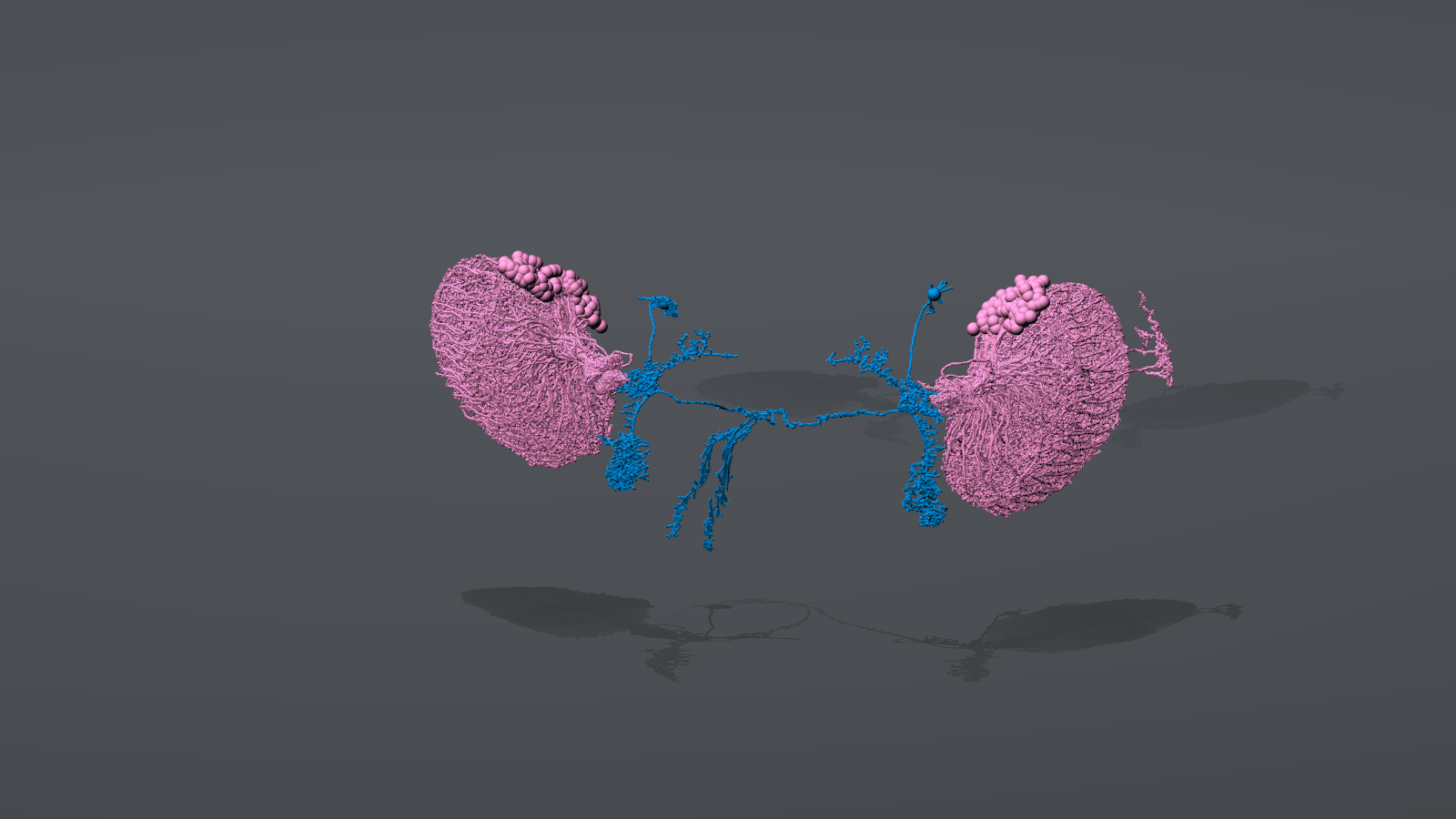
connkg quilt LPLC2 DNp01 --tubes --floor --still: the 210 LPLC2 neurons (reddish purple) and the two DNp01 neurons (blue), drawn as tubes, over the floor. See Reading the images.

connectomekg.scene.add_floor adds three things:

• A floor plane in the background gray, a little below the scene and far larger than the frame, so it fills the view behind the brain. The floor is only visible from a camera that looks down on it, which is why --floor defaults --elevation to 25 degrees.
• A key light: a spotlight high above the brain with a 75-degree cone that casts the shadows, plus a weak headlight so that shadowed surfaces stay readable.
• Shadow mapping at 8192 x 8192 pixels. At VTK's default of 1024, the shadows are visibly blocky at 4K, and a wide cone spreads the map over more floor. A narrower cone gives sharper shadows but shows its circular edge on the floor.

The floor is added after the camera is framed and after the depth report, because it reaches past the camera and would otherwise decide both. In the viewer, Cast to Looking Glass rebuilds the floor with the scene.

Skeletons drawn as lines cast almost no shadow. Add --tubes to a floored circuit view. Under the floor, line skeletons are rendered as GPU tubes either way: VTK's shadow pass can only shade lit geometry, and an unlit line's shader fails to compile, silently. The floor also re-orders the render passes so that translucent surfaces, the neuropil shells among them, are drawn after the shadowed floor rather than under it.

Shadow mapping adds a render pass for each frame, so the interactive viewer can respond more slowly with --floor. The stills and quilts are not affected in practice: a floored 4K still takes about 4 to 6 seconds.

Tuning constants

The visual constants live at the top of src/connectomekg/scene.py. Sizes are in world units, where the brain is about 8 units wide.

constant	value	controls
BACKGROUND	#5A5D62	default scene background
BACKGROUNDS	gray, charcoal, black, navy, light	named backgrounds for --background and the viewer
_FLOOR_STEP	0.24	how far a floor under a non-default background is shaded from it
_REFERENCE_FRAMED_NM	410,000	FAFB v783's framed extent, which marker sizes are scaled against
_MAX_MARKER_SCALE	4.0	cap on that scale
_CONTEXT_RADIUS	0.005	context sphere radius, circuit view
_FLOW_CONTEXT_RADIUS	0.014	context sphere radius, flow view
_FLOW_CONTEXT_STRIDE	10	flow view draws every Nth neuron
_CONTEXT_MUTE	0.45	how far context dot colors blend toward the background
_FLOW_CONTEXT_COLOR	#8A8F96	context dot color in the flow view, before muting
_SOMA_RADIUS, _FALLBACK_RADIUS	0.05, 0.09	soma and missing-skeleton spheres
_TUBE_RADIUS	0.01	skeleton tube radius with --tubes
_NEUROPIL_MAX_RADIUS	0.22	largest neuropil sphere
_FLOW_MAX_RADIUS, _FLOW_MIN_RADIUS	0.08, 0.004	flow tube radius range
_FLOW_BOW	0.15	tube bow, as a fraction of the distance between endpoints
_CONTEXT_DIM	0.85	darkening of idle neuropil spheres
_FLOW_AMBIENT	0.45	ambient share of the lighting on neuropil spheres and flow tubes
FLOOR_ELEVATION	25	default --elevation with --floor, degrees
_FLOOR_DROP, _FLOOR_SIZE	0.15, 120	floor distance below the scene, and its side length
_KEY_LIGHT_HEIGHT, _KEY_LIGHT_CONE	20, 75	key light height above the scene, and its cone in degrees
_KEY_LIGHT_INTENSITY, _FILL_LIGHT_INTENSITY	0.9, 0.35	key light and headlight intensity
_SHADOW_MAP_RESOLUTION	8192	shadow map size, pixels per side

Bounds on user input live in connectomekg.validation and apply equally to the CLI and the Python API:

bound	value
MAX_SCENE_NEURONS	500 neurons in a circuit
MAX_SKELETON_STEP	50
MAX_FLOW_PAIRS	500 tubes in a flow

Known limits

• Neuropil surfaces are FAFB v783 only. connkg meshes knows one mesh source. Another dataset renders without surfaces until its source is added to connectomekg.neuropil_meshes. BANC and MCNS therefore draw their cloud and flow in an unbounded space, with no brain shell around them.
• BANC and MCNS have no skeletons, so no circuit view. Their positions come from a soma table, not from traced geometry; see Soma positions for BANC and MCNS. The cloud and the flow view work; --view circuit has nothing to trace.
• somas=N reads 0 on BANC and MCNS. The counter reports has_soma, which only connkg skeletons writes, so it says nothing about these two releases even though every point in their cloud is a soma.
• Flow centroids still use marked points. The context cloud uses somas once connkg skeletons has back-filled them, and the circuit view has always read each soma from its skeleton, but the neuropil centroids in the flow view are still weighted over marked points.
• The soma back-fill needs the 31 GB download. A graph built without it draws the marked-point cloud, and connkg skeletons is the only thing that changes that.
• Large circuits are refused, not sampled. Narrow a SPEC that resolves to more than 500 neurons.

Use the scene from Python

build_brain_scene, aim_camera and add_floor are the steps connkg quilt runs, in the same order:

import pyvista as pv
from quiltwright import QUILT_PRESETS, render_quilt, save_quilt

from connectomekg import ConnectomeKG
from connectomekg.scene import FLOOR_ELEVATION, add_floor, aim_camera, build_brain_scene

spec = QUILT_PRESETS["16-landscape"].still(height=2160)
kg = ConnectomeKG("connectomes/fafb783")  # the dataset directory that holds .connectomekg/
plotter = pv.Plotter(
    off_screen=True, window_size=(round(spec.tile_height * spec.aspect), spec.tile_height)
)
info = build_brain_scene(plotter, kg, view="flow", specs=["LC4"], progress=print)
print(info.title, info.n_flow_pairs, info.n_flow_total)

aim_camera(plotter, info.points, fov=14.0, elevation=FLOOR_ELEVATION)
add_floor(plotter)
save_quilt(render_quilt(plotter, spec, fov=None), "renders/stills/flow_lc4", spec)
plotter.close()
kg.close()

To compute flow numbers without drawing anything, call connectomekg.scene.neuropil_flow(kg.store). See the scene API reference.